Compass Quantization
A raw bearing (0-359.999°) needs to become a label - N, NNE, NE, ... - for
d3.easygraph's
compassPoint16/compassPoint8/compassPoint4 utilities, using
the 16-, 8-, and 4-point compass
rose naming. Simple in principle - divide the circle into N equal sectors and see which one
the bearing falls in - but getting the sector boundaries right, and reconciling three different
resolutions cleanly, turned into a small, purely-for-fun math detour.
Sectors Have To Be Centered, Not Edged
The naive approach - floor(direction / sectorWidth) - puts a sector's boundary
exactly at 0°/N, splitting bearings just west and just east of due north into two different
sectors instead of both reading "N". The fix is a half-sector offset before flooring, so each
sector is centered on its own label: sector k of an N-point rose spans
[k * 360/N - 180/N, k * 360/N + 180/N). That's exactly what the three functions do,
each with its own sector width (22.5°, 45°, 90°) and half-width offset.
One Resolution Doesn't Reduce Cleanly To Another
It's tempting to compute only the finest (16-point) index and derive the coarser 8- and 4-point indices from it with a bitmask - cheaper than three independent formulas. It doesn't work in general. An even-numbered 16-sector sits exactly inside one 8-sector, so its index carries enough information. An odd-numbered 16-sector straddles an 8-point boundary at its own center - the same 16-index can come from either of its two neighboring 8-sectors, and that information is already gone once the bearing has been reduced to a 16-index. No formula of the 16-index alone, bitwise or otherwise, can recover it.
The Fix: Quantize To 32 First
The half-sector offset for the finest resolution in play (16 sectors, 22.5° wide) is 11.25° - exactly one 32nd of a circle. Dividing the circle into 32 raw, uncentered segments first gives a common fine-grained grid whose boundaries line up exactly with every centered sector boundary at all three resolutions, since 11.25 evenly divides 22.5, 45, and 90. Once a bearing is placed into one of the 32 segments, recovering each resolution's centered index is just a shift and a mask - no bearing math, no per-resolution formula, and (unlike deriving 8 from 16) no lost information, because 32 is finer than all three target resolutions rather than coarser:
_compassPoints = [
  'N', 'NNE', 'NE', 'ENE', 'E', 'ESE', 'SE', 'SSE',
  'S', 'SSW', 'SW', 'WSW', 'W', 'WNW', 'NW', 'NNW'
]

segment32(direction) = floor((direction + 360) / 11.25) & 0x1f

index16 = ((segment32 + 1) >> 1) & 0x0f
index8  = ((segment32 + 2) >> 1) & 0x0e
index4  = ((segment32 + 4) >> 1) & 0x0c
The shift amount for each resolution is that resolution's own half-sector offset, measured in 32nds: 11.25° (1 segment) for the 16-point rose, 22.5° (2 segments) for 8-point, 45° (4 segments) for 4-point. Verified exhaustively against the original per-resolution formulas at 0.01° resolution across -720° to 720° - zero mismatches.
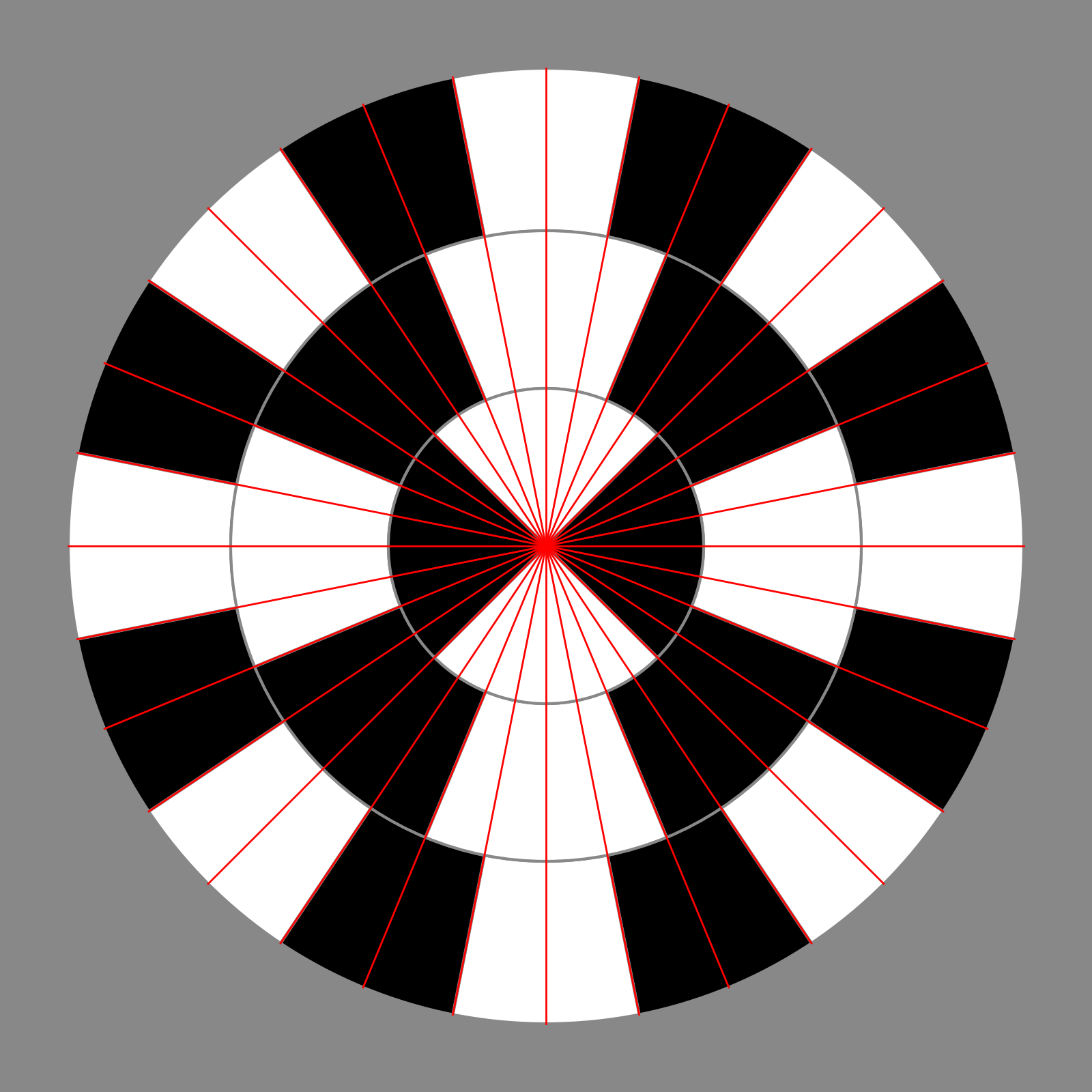
Direct, centered formulas - one per resolution.
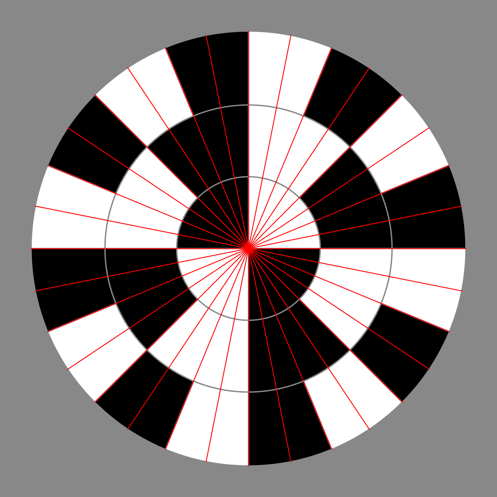
Same rings, each rotated by its own centering offset (1/32, 2/32, 4/32 of a circle).
Both images alternate black (odd sector) / white (even sector) per ring, sector 0/N centered
at the top. Rotating a centered sector by exactly half its own width cancels the centering -
[center - half, center + half) collapses back to the plain, edge-at-0
[k * width, (k + 1) * width) - so the second image is actually the naive,
uncentered quantization for all three resolutions, just drawn with the same 32 guide lines for
comparison.
That makes the second image's rings reduce cleanly into each other, unlike the first: since
22.5°, 45°, and 90° are exact multiples of 11.25° (2, 4, and 8 segments), masking
one bit off the outer (16-sector) ring's index gives exactly the middle (8-sector) ring's index,
and masking two bits gives the inner (4-sector) ring's - outer >> 1 == middle
and outer >> 2 == inner, holding exactly everywhere. That's the flip side of
"One Resolution Doesn't Reduce Cleanly To Another" above: the naive, uncentered quantization
reduces by simple bit-masking precisely because it throws away the centering that makes the
labels correct in the first place.
Converting Between The Two
Both images draw sector 0/N at the top rather than at 0°/east, matplotlib's own default - because a compass bearing (north = 0°, clockwise) and a standard math angle (east/+x axis = 0°, counterclockwise) are both just angles around the same circle, related by a fixed reflection rather than a rotation. Subtracting either one from 90° gives the other:
mathAngle = 90 - bearing
bearing   = 90 - mathAngle
The same formula both ways, since swapping which one you start from just reflects across the
same 45° line (NE/SW) again. In radians, feeding a bearing into something that expects a math
angle looks like angle = (bearingDegrees - 90) * Math.PI / 180 - exactly what
d3.easygraph.scatter's arrows feature expects for its angle
field (see the d3-easygraph README -
scatter deliberately stays geography-agnostic, so a caller with compass-bearing data, like the
wind arrows on weather's map, converts before handing points to it).
Wind Direction Is Reported Backwards (On Purpose)
METAR reports, and the meteorological convention generally, give wind direction as the bearing the wind is blowing from, not where it's headed - a reported 270° means a wind out of the west, blowing east. That's the right convention for a pilot lining up with a runway, but it reads backwards for a vector meant to show where the wind is actually going. Every place on this site that turns a stored bearing into a vector - the sin/cos decomposition below, and the wind arrow overlay on the weather map - flips it first:
towardDeg = fromDeg + 180
That's the whole fix - add 180°, nothing more - and it's applied once, up front, to the
raw bearing, before any of the averaging or decomposition below ever runs. Neither atan2
nor the sin/cos decomposition cares which convention fed it; the flip just isn't baked into either
formula, so it has to happen first.
Averaging Doesn't Work Either
A direction is an angle, not a plain number, so the usual sum / count average
breaks right where it matters most: two readings of 350° and 10° - both nearly due
north - naively average to (350 + 10) / 2 = 180°, due south, exactly backwards.
The fix is to stop averaging the angle directly and average it as a 2D unit vector instead:
ns = cos(d)   // north/south component
ew = sin(d)   // east/west component

meanDirection = atan2(sum(ew), sum(ns))
ns is cos and ew is sin - the reverse of
the usual x = cos(θ), y = sin(θ) pairing, for the same reason covered
above: a compass bearing measures from north (0°), not east, so north/south gets
cos and east/west gets sin, the opposite of a standard math angle.
Each direction becomes a point on the unit circle; combining north/south and east/west with
atan2 gives a mean that wraps correctly (350° and 10° now average to 0°,
as expected). No need to divide by the count first - atan2(y, x) is just
atan(y / x) with the division-by-zero case handled and the correct quadrant picked
from the sign of each argument, and scaling both arguments by the same count doesn't change their
ratio, so the raw sums work as well as the means would. The by-product
is as useful as the average itself: cos(d)/sin(d) is exactly the
north-south/east-west
decomposition weather and sensor data already needs for plotting - this site's report pages draw
wind not as a raw angle but as a vector in that same NS/EW space, and
bucket-series.js (the hourly/daily aggregation behind weather's and sensors' report
ribbons) uses this same circular mean for every bearing-named sensor, alongside a plain
sum / count average for everything else.
The two live report pipelines use the decomposition slightly differently, matching what each
actually needs from it. epw/report.php converts wind direction to sin/cos columns
before aggregating and keeps the resulting vector's own length -
sqrt(mean(ns)² + mean(ew)²) - as a free consistency signal: a
full-length vector means the wind held steady, a short one means it was averaged from readings
scattered all over the compass, not that it was calm. weather/sensors
instead force the averaged vector back onto the unit circle, since their consumers want a single
bearing to display, not a confidence magnitude.